Generalized Intersection over Union

A Metric and A Loss for Bounding Box Regression

Object Detection and $IoU$

Intersection over Union (IoU), also known as the Jaccard index, is the most popular evaluation metric for tasks such as segmentation, object detection and tracking. Object detection consists of two sub-tasks: localization, which is determining the location of an object in an image, and classification, which is assigning a class to that object.

The goal of localization in object detection is to draw a 2D bounding box around the objects in the scene. Further simplified in this example, we focus on a single bounding box. Click this button to .

The ground truth bounding box should now be shown in the image above. The source for this image and bounding box is the coco dataset. We know this is the ground truth because a person manually annotated the image. Now, click the button to show a prediction that might be made. This prediction bounding box is usually the output of a neural network, either during training or at inference time.

Explore what the or the look like. Intersection over Union ($IoU$) is then computed as follows:

$$IoU = \frac{|A\cap B|}{|A\cup B|} = \frac{|I|}{|U|}$$

Where A and B are the prediction and ground truth bounding boxes.

$IoU$ has the appealing property of scale invariance. This means that the width, height and location of the two bounding boxes under consideration are taken into account. The normalized IoU measure focuses on the area of the shapes, no matter their size.

Common Cost Functions

Object detection neural networks commonly use $\ell_1$-norm or $\ell_2$-norm for their cost function (aka. loss function). Our work shows that there is not a strong correlation between minimizing these commonly used losses and improving their IoU value.

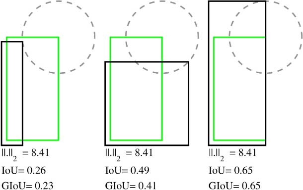
To understand why this is the case, recall that a rectangle can be represented parametrically in a variety of ways. For example, bounding boxes can be represented by their top-left corner $(x_1, y_1)$ and their bottom-right corner $(x_2, y_2)$, which can be written as $(x_1, y_1, x_2, y_2)$.

Alternatively, the $(x_c, y_c)$ coordinates for the center of the bounding box can be used in conjunction with the bounding box's width $w$ and height $h$ giving $(x_c, y_c, w, h)$.

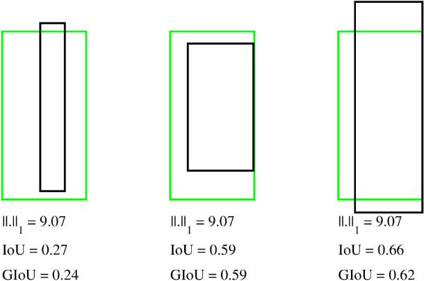
If we calculate $\ell_2$-norm distance, $||.||_2$ for the bounding boxes in both cases shown above and we calculate $\ell_1$-norm distance, $||.||_1$. Notice how the $\ell_n$-norm values are exactly the same, but their $IoU$ and $GIoU$ values are very different.

It is common practice to train a network by optimizing a loss function such as $\ell_1$-norm or $\ell_2$-norm, but then evaluate performance on a different function, such as $IoU$. Moreover, $\ell_n$-norm based losses are not scale invariant. Therefore, bounding boxes with the same level of overlap, but different scales will give different values. State of the art object detection networks deal with this problem by introducing ideas such as anchor boxes and non-linear representations, but even with these engineered tweaks, there is still a gap betwen the $\ell_n$-norm cost function and the $IoU$ metric.

$IoU$ vs. $GIoU$ as a Metric

In object detection, $IoU$ is used as a metric to evaluate how close the prediction bounding box is to the ground truth. In the first example above, the prediction and ground truth bounding boxes overlap, so the value for $IoU$ is non-zero. Let's look at an example where $IoU$ falls short.

First, . Now, say that instead of making a prediction like we saw above, what if we where the predicted bounding box has no overlap with the ground truth. In this case, and any other case where there is no overlap between the ground truth and prediction bounding boxes, intersection is 0, therefore $IoU$ will be 0 as well.

Now let's . Unfortunately, $IoU$ is still 0 for both. It would be nice if $IoU$ indicated if our new, better prediction was closer to the ground truth than the first prediction, even in cases of no intersection.

Our work proposes a solution to this, $GIoU$, which is formulated as follows:

$$GIoU = \frac{|A\cap B|}{|A\cup B|} - \frac{|C\backslash(A\cup B)|}{|C|} = IoU - \frac{|C\backslash(A\cup B)|}{|C|}$$

Where $A$ and $B$ are the prediction and ground truth bounding boxes. $C$ is the smallest convex hull that encloses both $A$ and $B$. Use the buttons below to visualize the value of $C$ for both of the predictions in this example.

Notice that the area of $C$ is smaller in the better case and all other values remain constant. $IoU$ will be 0 in both cases. Therefore, a smaller value is subtracted and the value of $GIoU$ increases as the prediction moves towards the ground truth.

vs.

$GIoU$ as a loss

Recall that in a neural network, any given loss function must be differentiable to allow for backpropagation. We see from the above example that in cases where there is no intersection, $IoU$ has no value and therefore no gradient. $GIoU$ however, is always differentiable.

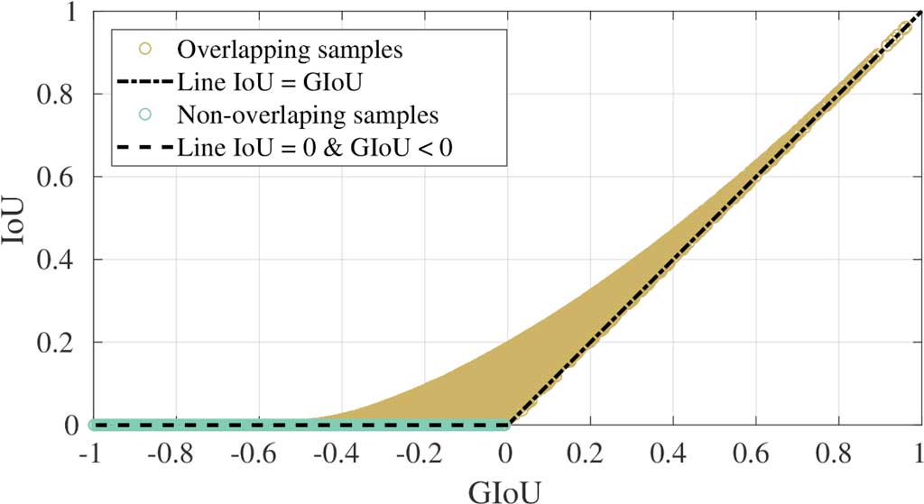
We sampled cases where the prediction bounding box overlaps (aka. intersects) the ground truth and cases where there is no intersection. The relationship between $IoU$ and $GIoU$ for these samples is shown in this figure.

From the plot, as from the formulation above, you can see that $GIoU$ ranges from -1 to 1. Negative values occur when the area enclosing both bounding boxes, e.g. $C$, is greater than $IoU$. As the $IoU$ component increases, the value of $GIoU$ converges to $IoU$.

$GIoU$ Algorithm

Pseudocode

Algorithm: $IoU$ and $GIoU$ as bounding box losses $input$: Predicted $B^p$ and ground truth $B^g$ bounding box coordinates: $B^p = (x^p_1,y^p_1,x^p_2,y^p_2) $, $B^g = (x^g_1,y^g_1,x^g_2,y^g_2)$ $output$: $\mathcal{L}_{IoU}$, $\mathcal{L}_{GIoU}$ 1. For the predicted box $B^p$, ensuring $x^p_2>x^p_1$ and $y^p_2>y^p_1$: $\hat{x}^p_1 = \min(x^p_1,x^p_2)$, $ \hat{x}^p_2 = \max(x^p_1,x^p_2)$, $\hat{y}^p_1 = \min(y^p_1,y^p_2)$, $\hat{y}^p_2 = \max(y^p_1,y^p_2)$ 2. Calculating area of $B^g$: $A^g = (x^g_2 - x^g_1)\times(y^g_2 - y^g_1)$ 3. Calculating area of $B^p$: $A^p = (\hat{x}^p_2 - \hat{x}^p_1)\times(\hat{y}^p_2 - \hat{y}^p_1)$ 4. Calculating intersection $\mathcal{I}$ between $B^p$ and $B^g$: $x^{\mathcal{I}}_1 = \max(\hat{x}^p_1,x^g_1)$, $x^{\mathcal{I}}_2 = \min(\hat{x}^p_2,x^g_2)$, $y^{\mathcal{I}}_1 = \max(\hat{y}^p_1,y^g_1)$, $y^{\mathcal{I}}_2 = \min(\hat{y}^p_2,y^g_2)$, $\mathcal{I} = \begin{cases} (x^{\mathcal{I}}_2 - x^{\mathcal{I}}_1) \times (y^{\mathcal{I}}_2 - y^{\mathcal{I}}_1) & \text{if} \quad x^{\mathcal{I}}_2 > x^{\mathcal{I}}_1, y^{\mathcal{I}}_2 > y^{\mathcal{I}}_1, \\ 0 & \text{otherwise} \end{cases}$ 5. Finding the coordinate of smallest enclosing box $B^c$: $x^{c}_1 = \min(\hat{x}^p_1,x^g_1)$, $x^{c}_2 = \max(\hat{x}^p_2,x^g_2)$, $y^{c}_1 = \min(\hat{y}^p_1,y^g_1)$, $y^{c}_2 = \max(\hat{y}^p_2,y^g_2)$ 6. Calculating area of $B^c$: $A^c = (x^c_2 - x^c_1)\times(y^c_2 - y^c_1)$ 7. $\displaystyle IoU = \frac{\mathcal{I}}{\mathcal{U}}$, where $\mathcal{U} = A^p+A^g-\mathcal{I}$ 8. $\displaystyle GIoU = IoU - \frac{A^c-\mathcal{U}}{A^c}$ 9. $\mathcal{L}_{IoU} = 1 - IoU$, $\mathcal{L}_{GIoU} = 1 - GIoU$

Team

Hamid Rezatofighi

Nathan Tsoi

Website

JunYoung Gwak

Amir Sadeghian

Ian Reid

Website

Silvio Savarese

Website

If you found this work helpful in your research, please consider citing:

@article{Rezatofighi_2018_CVPR,
  author    = {Rezatofighi, Hamid and Tsoi, Nathan and Gwak, JunYoung and Sadeghian, Amir and Reid, Ian and Savarese, Silvio},
  title     = {Generalized Intersection over Union},
  booktitle = {The IEEE Conference on Computer Vision and Pattern Recognition (CVPR)},
  month     = {June},
  year      = {2019},
}